gem-lte-core

GEM-LTE and Landreman’s analytic 3D equilibria: what connects, with the empirical fits

2026-10-21. A corrected companion to landreman_gfd_synthesis_framework.md, which is left unchanged for reference. Figure and code: basin_empirical.png, basin_empirical.py (the empirical counterpart of basin.py).

1. What Landreman (2026) establishes

M. Landreman, Analytic toroidal 3D MHD equilibria and steady Euler flows with invariant surfaces, arXiv:2609.26742 (v2, 2026-09-28); code at landreman/analytic_3d_equilibria.

• Equations. (∇×B)×B = ∇p, ∇·B = 0. Through (∇×B)×B = B·∇B − ∇|B|²/2, this is the same problem as steady, incompressible Euler flow with B as the velocity and a Bernoulli function in place of the pressure.
• Solutions. Explicit, non-axisymmetric fields in Cartesian coordinates, built from elementary functions, with exactly nested toroidal surfaces. Nothing is expanded in aspect ratio or departure from axisymmetry.
• Family 1: ι = 2 everywhere. Along a field line, with parameter ζ, the coordinates are decoupled harmonic oscillators, x″ = −x, y″ = −y, z″ = −4z. A field line is x = a cos ζ, y = b sin ζ, z = c cos(2ζ + β). The rotational transform is the frequency ratio of the oscillators: Δθ/Δφ = 4π/2π = 2.
• Family 2: sheared ι(ψ). The fields carry a vertical factor e^(−iλz). ι varies with the surface, and λ does not change it.
• Scope. The solutions are steady: no time dependence and no forcing. The motivation is counterexamples to Grad’s conjecture and test cases for fusion equilibrium codes. No geophysical application is discussed.
• AI involvement. The solutions were found with an AI model, GPT-6 Astra Pro, and every equation was checked by hand by the author.

2. Corrections to the earlier framework note

Claim in landreman_gfd_synthesis_framework.md	Status	Correction
A Beltrami condition (u ∥ B, force-free) makes MHD and the fluid equations map identically	Not what the paper uses	The solutions are not force-free. The Lorentz force is balanced by ∇p, and the fluid analogue is steady Euler flow with a Bernoulli function.
ι = ω_tidal / ω_annual	Asserted, not derived	In the paper, ι is the ratio of oscillator frequencies along a field line, a spatial winding ratio. Section 3 gives the GEM-LTE counterpart: a ratio of windings in the manifold.
Tidal forcing “re-anchors” the phase on the 3D torus	Not in the paper	The paper is steady. The time dependence comes only from GEM-LTE (section 3).
The pipeline of §6 and basin.py build Landreman surfaces	No	They build a generic helical torus. basin.py also mixes km and m, hence speeds of thousands of m/s. It is an illustration only.
“Together, they prove …”	Overstated	The correspondence is a structural analogy with one exact mathematical link (section 3), not a proof of a physical mechanism.
QBO as the axisymmetric k = 0 (Grad–Shafranov) case; ENSO as non-axisymmetric	Reasonable as a classification	Consistent with the QBO formulation (zonal mean, draconic–annual beat), but nothing in the paper is about the QBO or ENSO.

3. The exact link: the LTE response is a harmonic oscillator in the manifold

Chapter 12 (eq. 12-14) reduces Laplace’s tidal equations at the equator to

ζ(t) = sin(√A · M(t) + θ₀),

where M(t) is the tidally forced manifold. In time this obeys ζ″ − (M″/M′)ζ′ + A(M′)²ζ = 0, the reparametrization found in the September 2026 review of the chapter. Written in M instead of t, it is exactly

d²ζ/dM² = −A ζ,

a harmonic oscillator whose “time” is the manifold. The fitted model is a sum of such oscillators, sin(2π k F(t) + phase), on one manifold F(t), with windings k = h · k_base (integer harmonics h of a base winding) plus a few slow windings.

The correspondence with Landreman’s family 1 is then direct:

Landreman family 1	GEM-LTE fit
field-line parameter ζ	manifold, ζ = 2π k_base F(t)
x = a cos ζ, y = b sin ζ (the 1:1 pair)	the base winding
z = c cos(2ζ + β) (the 2:1 oscillator)	a harmonic h of the base: cos(h ζ + phase)
rotational transform ι = 2	ι = h = k_h / k_base
rational ι: closed field lines	integer harmonic ratios: the response repeats exactly in F
irrational ι: lines fill the surface	a slow winding with a non-integer ratio to the base
steady field	non-autonomous: F(t) moves back and forth along the line under tidal pacing

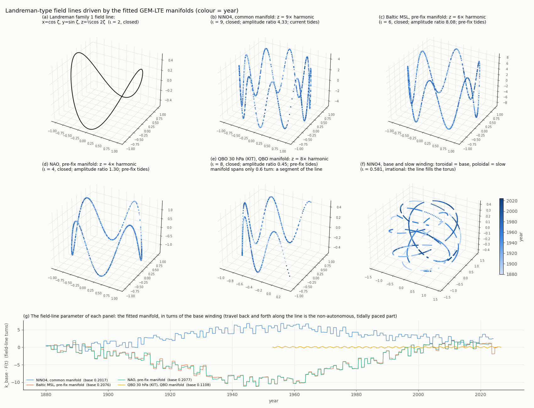
basin_empirical.py draws this literally. It takes each index’s fitted manifold, base term and dominant harmonic (fitted amplitudes and phases) and plots x = cos ζ, y = sin ζ, z = (A_h/A_base) cos(hζ + phase), coloured by year. Panel (a) is Landreman’s exact ι = 2 line for comparison. The field-line parameter itself, the manifold, is shown underneath.

What is new relative to the steady equilibria is the last row. In GEM-LTE the position along the invariant line is set by the tidally forced manifold, which drifts and steps every year (panel g). That is the non-autonomous part; Landreman’s solutions supply only the steady geometry it moves on.

4. Empirical rotational transforms from the fits

From the fitted windings (lt.exe.windings.N.json) of the multi-series runs in experiments/Oct2026_generator/legs/. “Dominant” is the largest term by squared amplitude. ι is its winding divided by the base.

Series	Manifold	Base k	Dominant ι (share)	Slow / base
NINO4, NINO3.4, NINO3, NINO1+2	common (current tides)	0.2017	9 (57–79%)	0.767
PDO, NINO4, IODE	common	0.2017	9 (25–41%)	0.581
PNA	common	0.2018	9 (37–42%)	0.571–0.578
SAM; Patagonia shelf SST	common	0.2017–0.2018	8 (37–62%)	0.571–0.672
AMO	common	0.2017	1 (26%), then 3 and 6	0.581
IODW	common	0.2017	3 (25%)	0.686
SOI and Darwin/Tahiti, monthly (fits with harmonics to ~250)	common	0.2018	227 (32–39%)	0.382–0.405
SOI, 5-day	common	0.2018	7 (44%)	0.382
QBO 30 hPa (KIT, ERA5)	QBO fit	0.1108	1 (48–55%), then 8	—
Baltic MSL	pre-fix tides, own manifold	0.2076	6 (64%)	0.593 (and 4.47)
NAO	pre-fix, own manifold	0.2077	4 (32%), then 1.71	1.71 (and 2.62)
AMO	pre-fix, own manifold	0.2076	slow 0.065 (41%), then 1	0.065 (and 1.69, 2.62)

Read this carefully. The integer values of ι are imposed by the model, which is built from integer harmonics of one base winding. What the data choose is (i) which harmonic dominates and (ii) the non-integer slow windings. So the table says that ENSO-type series sit on the ι = 9 line, the SAM and Patagonia SST on ι = 8, Baltic sea level on ι = 6 and the NAO on ι = 4, given the integer-harmonic model. The table alone does not show that the data prefer rational transforms; test 2 in section 7 checks that without the ladder, and finds they do for this base. The slow/base ratios are genuinely fitted. 0.57–0.59 recurs (the AMO/PDO/NINO4/IODE and PDO/PNA leg sets, and the independent pre-fix Baltic fit), but other leg sets give 0.67–0.77 or 0.38–0.41.

5. The other empirical findings, in this language

• One manifold, one field-line parameter. The leg fits share one manifold across records. In the correspondence above, that is a shared field-line parameter: different records are different harmonics, or different surfaces, along the same line. This is why a manifold held invariant is the foundation for judging excursions. Letting it vary per series gives each series its own parameter, so they no longer lie on a common line.
• Sensitivity grows with ι. Small changes in the manifold shift a winding’s phase in proportion to k. Between the pre-fix AMO, NAO and Baltic manifolds the shape differences are 35–70° of phase at the base winding (ι = 1) but several full turns at ι = 4–6. They come mostly from the half-year impulse amplitude (a 0.7% change gives about 100° at ι = 1). High-ι responses (the Baltic’s 6, ENSO’s 9) are therefore the ones that pin the manifold down, and the first to fail when it is slightly wrong. This parallels the sensitivity of high-ι surfaces to small changes in the equilibrium’s shape, but nothing beyond the parallel is claimed here.
• QBO as the axisymmetric case. The QBO fits treat the zonal mean (wavenumber 0) with a draconic–annual beat (experiments/Feb2026/QBO_FORMULATION.md). That matches the axisymmetric limit of the classification. The descending vertical phase of the QBO has a loose counterpart in family 2’s e^(−iλz) layering, where λ does not change ι. That is suggestive only; it has not been tested.
• Steady geometry, forced motion. Panel (g) of the figure is the non-autonomous content: the field-line parameter steps once a year at the tidal impulse and drifts over decades. Landreman’s equilibria are the curves those steps move along.

6. Limits

• Analogy, not equivalence. The exact statement is mathematical: the fitted response is a sum of oscillators in the manifold, which is the form of a family-1 field line. No spatial (3D) structure is fitted in GEM-LTE, so the toroidal geometry is not observed.
• Imposed integer transforms. In the fits, the integer ι come from the model’s harmonic ladder. Test 2 (section 7) finds the data favour integer multiples of this base without the ladder, but at a modest significance.
• Different manifolds. The current-tide and pre-fix manifolds differ, so ι values from different manifolds are comparable only as ratios within a fit.
• Steady versus forced. The paper says nothing about forcing; the forced part is GEM-LTE’s alone.

7. Tests (run 2026-10-21; landreman_tests.py, landreman_tests.png, landreman_tests.json)

Setup for tests 1 and 2:

• Model-free. Each record’s data, with a quadratic trend removed, are projected on sin(2πMF) for the common manifold of the AMO/PDO/NINO4/IODE fit (base 0.2017, slow winding 0.1173 = 0.581 × base), with no harmonic ladder.
• Records. Only data not used to fit that manifold: 89 Kaplan quads, 14 other indices and 60 tide gauges. The “independent” subset (128 records) also excludes any record whose detrended data correlate |r| > 0.5 with AMO, PDO, NINO4 or IODE.
• Null. 200 surrogates per record with the same spectrum and scrambled phases, projected on the same manifold.

1. Common slow-winding ratio: not supported.
   • Only 1% of independent records have their strongest sub-base winding within ±0.004 of 0.1173 (ratio 0.581), against 5% for surrogates.
   • The densest cluster is at ratio 0.93, which is the low shoulder of the base winding’s own peak (it also appears in the surrogates). The tide gauges alone cluster at 0.347 (p = 0.005), which is not the fitted slow ratio.
   • So 0.58 is a property of particular fits, not of the data in general.
2. Integer multiples of the base in the data: supported.
   • Independent records have more power within ±0.01 of h × 0.2017 (h = 1–9) than their surrogates: mean percentile 76, with 38 of 128 above the 95th percentile (6.4 expected). Quads, indices and tide gauges each show it separately: 71, 83 and 82.
   • It is specific to the base: of 45 base windings from 0.150 to 0.260, the best are 0.2000 and 0.2025.
   • It is specific to integers: half-integer multiples score below chance (42).
   • It is not the seasonal cycle: removing each record’s monthly climatology changes nothing (76.2).
   • Significance. Neighbouring records share signal, so the scores of wrong bases scatter between 32 and 69, far more than independent records would allow. The fair statement is that 0.2017 is the best of 45 bases in data that did not set it (roughly p ≈ 0.02–0.04), not the formal z ≈ +10.
   • In the language of section 3, the data do prefer the rational surfaces (integer ι) of this base winding, beyond what the model imposes. Rational, closed field lines are what Landreman’s family 1 has everywhere (ι = 2).
3. Sheared ι for the QBO across 70/50/30 hPa: no evidence, and the model-free version is inconclusive.
   • The three fitted runs have the same base winding (0.1100, 0.1111, 0.1108), which carries 64%, 96% and 55% of the KIT response. That points to a uniform transform, not a sheared one. Their secondary harmonics differ (26×, 2×, 8×), but those runs were seeded from one another.
   • Model-free, the strongest data ridge on a common QBO manifold moves from M ≈ 0.16 (30 hPa) to 0.49 (50 hPa) and 0.75 (70 hPa). But only the 30 hPa ridge is stable between the two halves of the record, and the QBO manifold spans only 0.6 turns of its base, too little to resolve windings that close together. So this test cannot decide the question.

8. MHD and rotating-fluid factors: what the tidal forcing drives poloidally and toroidally (2026-10-22)

The premise of GEM-LTE is that tidal forcing, not wind, supplies the energy that makes up the basin’s losses. Wind cannot be separated into cause and effect, so this section maps the stellarator picture onto the rotating, gravitating fluid with the forcing taken to be tidal only.

8.1 The chain of equivalences

• MHD equilibrium = steady Euler flow (exact, Landreman). (∇×B)×B = ∇p is the same equation as (∇×u)×u = −∇H, with B ↔ velocity u, current J = ∇×B ↔ vorticity ω, and p ↔ −H (the Bernoulli function).

• Adding rotation and gravity (the Laplace tidal equations are the shallow-layer form):

  (ω + 2Ω) × u = −∇(

  u

  ²/2 + gη + U) + losses

  The “current” becomes the absolute vorticity ω + 2Ω, so planetary rotation acts as a strong, uniform background current. The “pressure” becomes the Bernoulli function, which contains the tidal potential U.

8.2 The equivalent factors

MHD (stellarator)	Rotating fluid / LTE	In GEM-LTE
magnetic field B	velocity u (Alfvén scaling B/√(μ₀ρ))	response amplitude, sin(k·F)
current J = ∇×B	absolute vorticity ω + 2Ω	Coriolis terms 2Ω sin φ in eqs. 12-1 and 12-2
pressure p	−H = −(gη + |u|²/2 + U)	ζ and the tidal potential U
Lorentz force J×B	Coriolis plus vortex force, (ω+2Ω)×u	the coupling terms −v·2Ω sin φ and +u·2Ω sin φ
flux surfaces ψ = const	Bernoulli / potential-vorticity surfaces	the manifold F as the surface label (section 3)
frozen-in flux (ideal MHD)	Kelvin’s circulation theorem / PV conservation	invariant manifold
resistivity	friction and viscosity	the losses the tidal forcing must make up
vacuum field of external coils (∇×B** = 0)**	tidal force −∇U (curl-free)	the forcing that builds F
rotational transform ι	poloidal circuits per toroidal circuit of a parcel	so far only a ratio of windings in F (section 4)
Lundquist number (transport / diffusion)	quality factor, forcing period / damping time	fitted damping (mp)

The coil row is the key correspondence. A stellarator gets its rotational transform from external coils whose vacuum field is curl-free, without a net plasma current. The tidal force is likewise an external, curl-free field. The forced, wind-free premise is therefore the fluid analogue of a stellarator, not a tokamak, whose transform comes mostly from current driven inside the plasma (the analogue of wind-driven vorticity).

8.3 Poloidal versus toroidal: what the tidal forcing drives

Geometry as in basin.py: toroidal = along the basin (east–west at the equator, zonal flow u); poloidal = the cross-section (north–south and vertical, v and w: meridional overturning and upwelling).

1. The long-period tides drive only the poloidal direction.
   • The forcing used here (Mm, Mf and the aliased lunar periods the manifold is built on) is degree-2, order-0. Its potential U ∝ P₂(sin φ) does not depend on longitude, so ∂U/∂λ = 0 and the zonal (toroidal) tractive force is exactly zero.
   • The force is purely meridional, −(g/a)·∂η/∂φ ∝ sin φ cos φ: zero at the equator, with its largest gradient there, so near the equator it acts as a meridional convergence or divergence. Size: about 2 × 10⁻⁸ m/s² for Mf at 5° (equilibrium-tide amplitude roughly 4 cm).
2. The toroidal amplitude comes from two conversions.

   • Coriolis turning (the analogue of the dynamo Ω-effect). Eq. 12-1, ∂u/∂t = +2Ω sin φ·v − (g/(a cos φ))·∂ζ/∂λ, with ∂U/∂λ = 0: the first term converts poloidal flow v into toroidal flow u with a gain of about f/ω = 2Ω sin φ/ω. In the LTE derivation φ is the tidally driven latitude excursion φ(t) of eq. 12-13, so 2Ω sin φ(t) ≈ 2Ω·φ(t) is the poloidal-to-toroidal conversion factor: the same excursion that builds the manifold sets how much of the response becomes zonal. In MHD, differential rotation does this by shearing poloidal field into toroidal field.

     Latitude	f/ω for Mf	f/ω for Mm
     equator	0	0
     2°	≈ 1	≈ 1.9
     5°	≈ 2.4	≈ 4.8

   • The basin boundaries. The zonal pressure-gradient term −g·∂ζ/∂λ exists only because the coasts break the zonal symmetry: the standing mode SW(s) of eq. 12-7. For the QBO’s zonal ring (k = 0) the term vanishes, which is why the QBO is the axisymmetric case.

3. The result is a two-band structure.
   • Within the equatorial deformation radius, √(c/β) ≈ 330 km or about 3° (c ≈ 2.5 m/s), rotation cannot convert the flow: the response stays divergent and equatorially guided (Kelvin dynamics, poloidal-dominated).
   • Farther from the equator the conversion is effective and the response becomes rotational (Rossby dynamics, toroidal-dominated).

8.4 Empirical support so far (ENSO)

• Pinned standing mode (enso_spatial_mode.py, .png, .json; model-free projection of each location on the windings of the common manifold, 1950–2022):
  • For the significant windings (9× and 3× most strongly, then 4×, 6×, 1×), every equatorial location from 170°E to 90°W, including all four Niño regions, has the same phase within about ±20°, with a node near 160°E and the western Pacific opposite. No location shows a phase drifting with longitude: standing, not travelling.
  • Darwin pressure is in phase with Niño3.4 SST and Tahiti opposite (within 10° at 1×, 3×, 9×): the SOI see-saw is the same mode.
  • 9×, 3×, 4× have the eastern (canonical) shape; 1×, 6× and the slow winding the central-Pacific shape.
  • Between 1950–1986 and 1987–2022 the spatial pattern is kept while its timing against the manifold shifts in common (about −60° at 9×).
• Thermocline circuit (enso_subsurface_d20.py, .png; ORAS5 depth of the 20 °C isotherm 1958–2022, data from experiments/Oct2026_generator/ORAS5/fetch_d20.py):
  • The two bands of 8.3 appear in the data: the anomaly migrates eastward along the equator (about 0.3 m/s) and westward at 5–8° (about 0.2–0.3 m/s). These are slow heat-content migrations, not free wave speeds.
  • The tidally forced Niño3.4 model reproduces the zonal tilt (east +0.53, west −0.57 at lag 0), slightly beyond what its SST fit implies (west z = −3.4 against imitators built from observed Niño3.4 plus noise at the same r = 0.73).
  • It does not reproduce the recharge precursor: the western thermocline deepening about a year ahead of the Niño3.4 peak (+0.05 vs +0.17 for imitators, +0.24 observed). That is the off-equatorial return leg of the circuit, the poloidal part of the stellarator picture.

8.5 What is exact and what is analogy

• Exact: Landreman’s MHD–Euler equivalence; the ω + 2Ω and Bernoulli substitutions; the zero zonal force of order-0 tides; the Coriolis conversion term of the Laplace equations.
• Analogy: Coriolis as the Ω-effect; the tide as the coil field; the wave branches (equatorial Kelvin ↔ the compressional, fast-magnetosonic branch; Rossby ↔ the shear, Alfvénic branch, with rotational stiffness in place of field-line tension). The ocean is forced and dissipative, not an ideal equilibrium, and carries known shear instabilities (tropical instability waves, 20–40 days).
• Not yet measured: a physical ι, poloidal circuits per toroidal circuit of a water parcel. That needs 3D currents (zonal u and meridional v at depth along the equator) from ORAS5, and would turn ι from a ratio of windings into a measured quantity. A two-leg fit of Niño3.4 with the warm-water volume (5°S–5°N mean D20) would test whether tidal forcing reaches the recharge leg at all.